
Understanding Linear Regression -Part 2


INTRODUCTION
Wow ! Another interesting day to continue learning our first ML algorithm, yay! I hope you have read Understanding Linear Regression -Part 1 ? Today, we will be wrapping up with everything under Linear Regression.
Table of Contents
What is Gradient Descent?
Overview of Multiple Linear Regression
Assumption of Linear Regression
What is Gradient Descent?
Gradient descent is an iterative optimization algorithm to find the minimum of a function. Here, that function refers to the Loss function.
Also on using Gradient descent, the term learning rate comes into the picture. The learning rate is denoted by α and this parameter controls how much the value of m and c should change after each iteration/step.For different values of m and c, we will get different error values as shown in Figure 1 below.

Figure 1 : Cases of Learning Rate
Starting with an initial value of m and c as 0.0 and setting a small value for the learning rate e.g. α=0.001, for this value we calculate the error value using our loss function. For different values of m and c, we will get different error values as shown in figure 2.
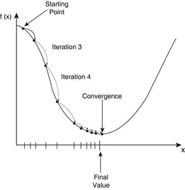
figure 2 : Working of Gradient Descent (Simple Linear Regression)
Once the initial values are selected, we then find the partial derivative of the loss function by applying the chain rule.
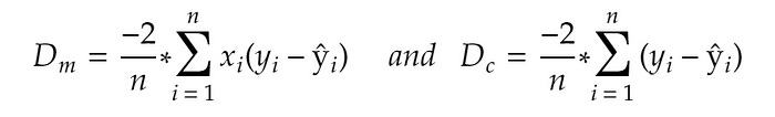
Figure 3: Partial derivatives (Slopes) of loss function
Once the slope is calculated, we now update the value of m and c using the formula shown in Figure 4.
Figure 4: Formula for updating m and c
If the slope at the particular point is negative then the value of m and c increases and the point shifts towards the right side by a small distance as seen in Figure 2.
If the slope at the particular point is positive then the value of m and c decreases and the point shifts towards the left side by a small distance.
The Gradient descent algorithm keeps on changing the value of m and c until the loss becomes very small or becomes 0 (ideally) and this is how we find our Best Fit Regression Line.
Gradient representation of Gradient descent ||source
Now that you have understood the complete working of the Simple Linear Regression algorithm, let’s see how the Multiple Linear Regression algorithm works.
Overview of Multiple Linear Regression
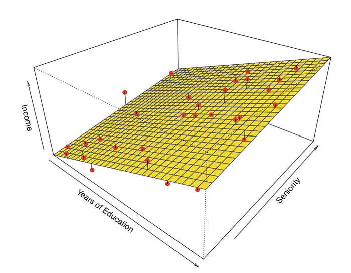
Figure 5: Multiple Linear Regression(Graph)
In real-life scenarios, there will never be a single feature that predicts a target. Hence, we simply perform multiple linear regression.
The equation below shows is very similar to the equation for simple linear regression; simply add the number of independent features/predictors and their corresponding coefficients.
Note: The working of the algorithm remains the same, the only thing that changes is the Gradient Descent graph. In Simple Linear Regression, the gradient descent graph was in 2D form, but as the number of independent features/predictors increases, the gradient descent graph’s dimensions also keep on increasing.
Figure 6 shows a Gradient Descent graph in a 3D format where A is the initial weight/starting point and B is the global minima.
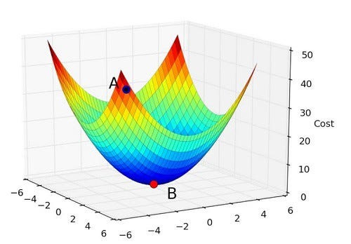
Figure 6: Gradient Descent (Multiple Linear Regression)
Figure 7 shows the complete working of the Gradient Descent in 3D format from A to B.
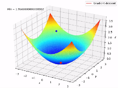
Figure 7: Working of Gradient Descent (Multiple Linear Regression )
Assumptions of Linear Regression
The following are the fundamental assumptions of Linear Regression, which can be used to answer the question of whether we can use a linear regression algorithm on a particular dataset?
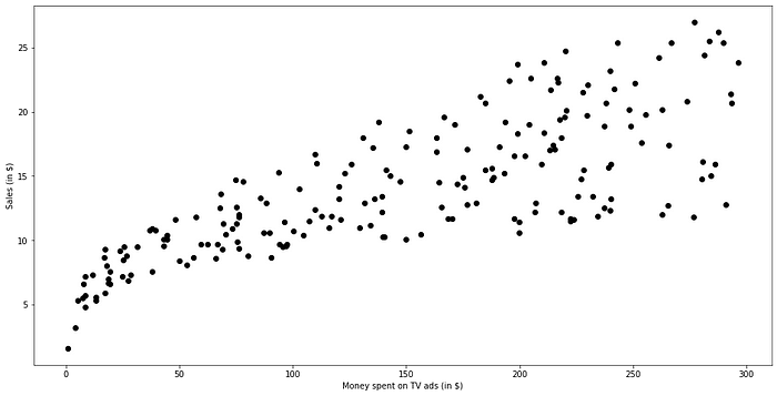
A linear relationship between features and the target variable:
Linear Regression assumes that the relationship between independent features and the target is linear. It does not support anything else. You may need to transform data to make the relationship linear (e.g. log transform for an exponential relationship).
Example of Linear Relationship
Little or No Multicollinearity between features:
Multicollinearity exists when the independent variables are found to be moderately or highly correlated. In a model with correlated variables, it becomes a tough task to figure out the true relationship of predictors with the target variable. In other words, it becomes difficult to find out which variable is actually contributing to predict the response variable.
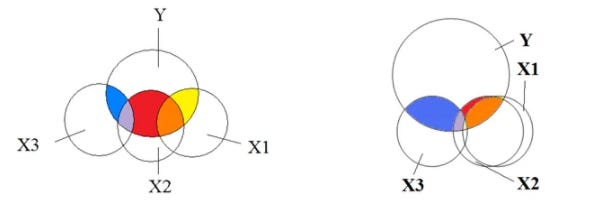
Example of Multicollinearity
Little or No Autocorrelation in residuals:
The presence of correlation in error terms drastically reduces the model’s accuracy. This usually occurs in time series models where the next instant is dependent on the previous instant. If the error terms are correlated, the estimated standard errors tend to underestimate the true standard error.No Heteroscedasticity(Constant Variance of Errors):
The presence of non-constant variance in the error terms results in heteroscedasticity. Generally, non-constant variance arises in the presence of outliers. Looks like, these values get too much weight, thereby disproportionately influences the model’s performance.
Normal distribution of error terms:
If the error terms are not normally distributed, confidence intervals may become too wide or narrow. Once the confidence interval becomes unstable, it leads to difficulty in estimating coefficients based on the least-squares. The presence of non-normal distribution suggests that there are a few unusual data points that must be studied closely to make a better model.
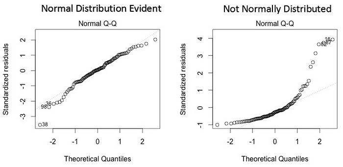
Example of Normal distribution of error terms
References
Linear Regression for Machine Learning
Linear Regression using Gradient
That’s all folks ! Get ready for our next article on logistics Regression.
 | A guest post by
|