The Gaussian Distribution

Let's discuss the Gaussian Distribution in Probability and Machine Learning

We’ve reached a check point. The end of our coverage on probability. Over the past days, we’ve highlighted and explored the concept of `probability` with focus on how it influences Machine Learning. We shall round up this subject by looking at the Gaussian distribution. Through this, we shall see what distribution are, and how applicable they are in our field of study. Let’s get in <3

Understanding Distributions in Machine Learning

In statistics and machine learning, distributions describe how data is spread or distributed. When we say a dataset follows a certain distribution, we mean that the data behaves in a particular pattern or shape. Let’s break down a common distribution, the famous…

Gaussian (Normal) Distribution.

Imagine you’re measuring the heights of a large number of people. Most people will be of average height, while fewer will be extremely tall or short. When you plot these heights on a graph (with height on the x-axis and frequency on the y-axis), you get a bell-shaped curve known as the Gaussian distribution.

Characteristics of this graph would include -

• Bell-Shaped Curve: The graph is symmetric around the mean (average value).

• Mean, Median, and Mode are equal: In a perfect Gaussian distribution, the mean (average), median (middle value), and mode (most frequent value) are all the same.

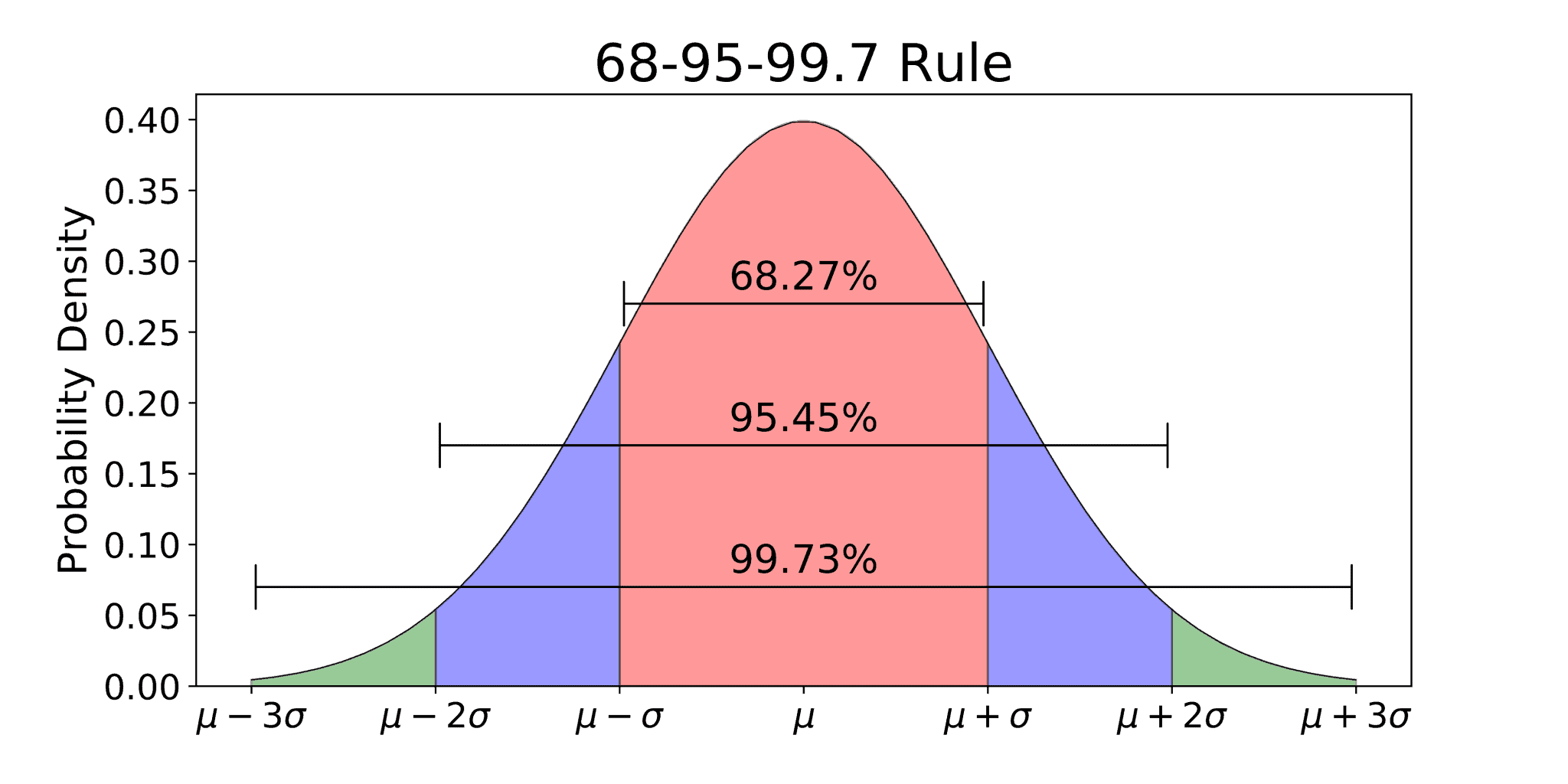
• The `68-95-99.7` Rule - which means that…

  • 68% of data falls within 1 standard deviation (σ) of the mean.

  • 95% falls within 2 standard deviations.

  • 99.7% falls within 3 standard deviations.

The Gaussian distribution can be represented with the following formula -

\(f(x) = \frac{1}{\sqrt{2 \pi \sigma^2}} \exp \left( -\frac{(x - \mu)^2}{2 \sigma^2} \right) \)

Where:

• x is the data point

• μ is the mean

• σ is the standard deviation

• exp⁡ denotes the exponential function

Let’s break it down even further…

• x (Data Point):

  • This is the value for which you are calculating the probability. In the context of our heights example, x could represent a specific person's height.

• μ (Mean):

  • The mean (average) of the dataset. Think of it as the "center" of our bell curve. For the heights example, it would be the average height of all the people in the dataset.

  • The graph is symmetric around this point, meaning most data points are close to the mean.

• σ (Standard Deviation):

  • The standard deviation measures the spread or dispersion of the data. It tells us how much the data varies from the mean.

  • A smaller σ means the data points are tightly clustered around the mean, creating a "narrow" bell curve.

  • A larger σ means the data points are more spread out, creating a "wider" bell curve.

• exp -

  \(exp\left(-\frac{(x - \mu)^2}{2\sigma^2}\right) \)

  • The exponential function. This part decreases the probability as xxx moves away from the mean, creating the "tails" of the curve.

  • It measures how far the data point x is from the mean. If x is far from μ (the mean), this value becomes large, making the probability smaller.

  • As a result, the further x is from the mean, the smaller the probability, creating the "tails" of the bell shape.

• \(\frac{1}{\sqrt{2 \pi \sigma^2}} \\)

  This part ensures that the total area under the curve is equal to 1, making it a proper probability distribution.

• It acts like a "normalization factor" that adjusts the height of the curve based on the standard deviation.

Think of the Gaussian formula as a way of telling us how "likely" different values are -

• The values near the mean are more likely, so they get higher probabilities, creating the peak.

• As you move away from the mean, the likelihood of those values decreases, creating the slope and tails of the curve.

This pattern of probabilities forms the familiar smooth, bell-shaped curve known as the Gaussian distribution.

Why Does This Matter for Machine Learning?

• Understanding Data Patterns - Knowing how data behaves can help us choose the right algorithms.

• Making Predictions - Many machine learning techniques assume data follows a normal distribution.

• Performing Statistical Tests - These tests often rely on data following certain distributions.

We may have a taken a leap into some more statistics-oriented concepts like.. the Standard deviation. But we shall revisit these in our next drive through `Statistics for Machine Learning`.

So don’t get confused. Seek additional resource and read over again, if need be.

Cheers. Happy Learning!